Forest Canopy Dimensions and Statistical Validation¶

Jupyter notebook

This page was rendered from the stored outputs of 3_canopy_statistical_validation.ipynb as of 2026-07-13; it is not executed at build time.

View on GitHub · Open in nbviewer · Open in Colab · Raw .ipynb

Kernel: Python 3 (ipykernel) · Environment: Python 3 with numpy, scipy, pandas and matplotlib · Companion page: metabolic-scaling/results/

Part II: Metabolic Scaling Theory and Biological Fractals

Overview¶

This notebook supports the Results section "Table 4: Forest Canopy Height Model Dimensions" and the "Statistical Validation" section. Metabolic scaling theory predicts that space-filling biological resource-distribution networks have a mass (self-affine) dimension near \(d = 3/2\). The manuscript measured the differential box-counting (DBC) mass dimension of LiDAR canopy height models (CHMs) across six forest types, then pooled the leaf, branch/root, and canopy measurements to test agreement with \(d = 3/2\).

Here we (1) reproduce Table 4 exactly, (2) compute the canopy group mean and dispersion, and (3) run formal statistical tests — one-sample \(t\)-tests and TOST equivalence tests — of each group and the pooled data against the \(d = 3/2\) prediction, reporting the results honestly.

1. Published Table 4 (reference values)¶

Transcribed directly from the manuscript. Each CHM is a LiDAR-derived raster of roughly \(3.6\times10^5\) px; \(d_M\) is the FracLac DBC mass dimension with the predicted value \(3/2\).

import numpy as np
import pandas as pd
import matplotlib.pyplot as plt
from scipy import stats

# Table 4 - forest canopy height model (CHM) mass dimensions (FracLac DBC), predicted d_M = 3/2
table4 = pd.DataFrame([
    ["Lowland Rainforest",   361201, 1.3313, 0.9860],
    ["Pine/Hardwood SC",     362403, 1.5223, 0.9898],
    ["Sierra Madre Oaks AZ", 362404, 1.4973, 0.9886],
    ["Western Ponderosa NM", 361802, 1.4566, 0.9847],
    ["SW Mixed Conifer NM",  361802, 1.5319, 0.9869],
    ["SW Spruce-Fir NM",     361802, 1.5355, 0.9862],
], columns=["Site","Pixels","d_M","mu_r2"])

# leaf and branch/root values from Tables 2 and 3 (for pooled validation)
leaf_vals   = np.array([1.5384, 1.4844, 1.5525, 1.5135, 1.5083])
branch_vals = np.array([1.4946, 1.4775, 1.4549])
canopy_vals = table4["d_M"].values

pd.set_option("display.float_format", lambda v: f"{v:.4f}")
print("TABLE 4 - Forest canopy height model mass dimensions")
print(table4.to_string(index=False))
print()
cm = canopy_vals.mean(); csd = canopy_vals.std(ddof=1); cse = csd/np.sqrt(len(canopy_vals))
print(f"Canopy mean = {cm:.4f}   SD = {csd:.4f}   SE = {cse:.4f}")
print(f"Manuscript reports canopy 1.479 +/- 0.080  ->  matches (mean {cm:.3f}, SD {csd:.3f})")

TABLE 4 - Forest canopy height model mass dimensions
                Site  Pixels    d_M  mu_r2
  Lowland Rainforest  361201 1.3313 0.9860
    Pine/Hardwood SC  362403 1.5223 0.9898
Sierra Madre Oaks AZ  362404 1.4973 0.9886
Western Ponderosa NM  361802 1.4566 0.9847
 SW Mixed Conifer NM  361802 1.5319 0.9869
    SW Spruce-Fir NM  361802 1.5355 0.9862

Canopy mean = 1.4791   SD = 0.0781   SE = 0.0319
Manuscript reports canopy 1.479 +/- 0.080  ->  matches (mean 1.479, SD 0.078)

2. Group summary statistics¶

We assemble the three measurement groups — leaves (Table 2), branch/root (Table 3), and canopy (Table 4) — and compute each group's mean, standard deviation, and standard error, comparing to the manuscript's reported values (leaf \(1.519\), branch \(1.476\), canopy \(1.479\)).

def group_stats(x):
    n = len(x); return n, x.mean(), x.std(ddof=1), x.std(ddof=1)/np.sqrt(n)

rows = []
for label, arr, reported in [("Leaf", leaf_vals, "1.519 +/- 0.027"),
                             ("Branch/Root", branch_vals, "1.476 +/- 0.020"),
                             ("Canopy", canopy_vals, "1.479 +/- 0.080")]:
    n, m, sd, se = group_stats(arr)
    rows.append([label, n, round(m,4), round(sd,4), round(se,4), reported])
summary = pd.DataFrame(rows, columns=["Group","n","mean","SD","SE","manuscript (mean +/- SD)"])
print(summary.to_string(index=False))
print()
print("All three computed means reproduce the manuscript's reported values;")
print("the reported '+/-' is the sample standard deviation in every case.")

      Group  n   mean     SD     SE manuscript (mean +/- SD)
       Leaf  5 1.5194 0.0266 0.0119          1.519 +/- 0.027
Branch/Root  3 1.4757 0.0199 0.0115          1.476 +/- 0.020
     Canopy  6 1.4792 0.0781 0.0319          1.479 +/- 0.080

All three computed means reproduce the manuscript's reported values;
the reported '+/-' is the sample standard deviation in every case.

3. One-sample \(t\)-tests against \(d = 3/2\)¶

The classical null-hypothesis test asks whether each group mean differs from \(1.5\). Failing to reject \(H_0\) is not proof of equivalence — it can simply reflect low power with small \(n\) — which is why we follow with an equivalence test in section 4.

print("One-sample t-tests of each group mean against the MST prediction d = 3/2:")
print()
for label, arr in [("Leaf", leaf_vals), ("Branch/Root", branch_vals), ("Canopy", canopy_vals)]:
    t, p = stats.ttest_1samp(arr, 1.5)
    verdict = "reject (differs from 1.5)" if p < 0.05 else "cannot reject (consistent with 1.5)"
    print(f"  {label:12s} n={len(arr)}  mean={arr.mean():.4f}  t={t:+.3f}  p={p:.4f}  -> {verdict}")
print()
pooled = np.concatenate([leaf_vals, branch_vals, canopy_vals])
t, p = stats.ttest_1samp(pooled, 1.5)
print(f"  POOLED (all 14):  mean={pooled.mean():.4f}  t={t:+.3f}  p={p:.4f}")
print(f"  -> pooled mean is statistically indistinguishable from 1.5 (p={p:.3f}).")

One-sample t-tests of each group mean against the MST prediction d = 3/2:

  Leaf         n=5  mean=1.5194  t=+1.630  p=0.1785  -> cannot reject (consistent with 1.5)
  Branch/Root  n=3  mean=1.4757  t=-2.116  p=0.1685  -> cannot reject (consistent with 1.5)
  Canopy       n=6  mean=1.4791  t=-0.654  p=0.5422  -> cannot reject (consistent with 1.5)

  POOLED (all 14):  mean=1.4928  t=-0.489  p=0.6333
  -> pooled mean is statistically indistinguishable from 1.5 (p=0.633).

4. TOST equivalence test against \(d = 3/2\)¶

The two one-sided tests (TOST) procedure reverses the burden of proof: the null hypothesis is non-equivalence, and rejecting it establishes that the mean lies within a pre-set equivalence margin \([1.5-\delta,\ 1.5+\delta]\). We test margins \(\delta = 0.10\) and the stricter \(\delta = 0.05\).

\[t_{\text{lower}} = \frac{\bar{x} - (1.5-\delta)}{\mathrm{SE}}, \qquad t_{\text{upper}} = \frac{\bar{x} - (1.5+\delta)}{\mathrm{SE}}\]

Equivalence is declared when both one-sided tests reject, i.e. \(\max(p_{\text{lower}}, p_{\text{upper}}) < \alpha\).

def tost(arr, mu=1.5, margin=0.1):
    """Two one-sided tests for equivalence within [mu-margin, mu+margin].
       Returns the (larger) of the two one-sided p-values; p < alpha => equivalent."""
    n = len(arr); mean = arr.mean(); se = arr.std(ddof=1)/np.sqrt(n); df = n-1
    low, high = mu-margin, mu+margin
    t_low  = (mean-low)/se;  p_low  = stats.t.sf(t_low, df)    # H0: mean <= low
    t_high = (mean-high)/se; p_high = stats.t.cdf(t_high, df)  # H0: mean >= high
    return max(p_low, p_high)

print("TOST equivalence tests against d = 3/2 (alpha = 0.05):")
print()
for margin in [0.10, 0.05]:
    print(f"  Equivalence margin +/- {margin}:")
    for label, arr in [("Leaf", leaf_vals), ("Branch/Root", branch_vals),
                       ("Canopy", canopy_vals), ("POOLED", pooled)]:
        p = tost(arr, 1.5, margin)
        verdict = "EQUIVALENT to 3/2" if p < 0.05 else "not shown equivalent"
        print(f"    {label:12s} TOST p = {p:.4f}  ->  {verdict}")
    print()

TOST equivalence tests against d = 3/2 (alpha = 0.05):

  Equivalence margin +/- 0.1:
    Leaf         TOST p = 0.0012  ->  EQUIVALENT to 3/2
    Branch/Root  TOST p = 0.0112  ->  EQUIVALENT to 3/2
    Canopy       TOST p = 0.0279  ->  EQUIVALENT to 3/2
    POOLED       TOST p = 0.0000  ->  EQUIVALENT to 3/2

  Equivalence margin +/- 0.05:
    Leaf         TOST p = 0.0311  ->  EQUIVALENT to 3/2
    Branch/Root  TOST p = 0.0776  ->  not shown equivalent
    Canopy       TOST p = 0.2013  ->  not shown equivalent
    POOLED       TOST p = 0.0062  ->  EQUIVALENT to 3/2

5. Combined forest plot¶

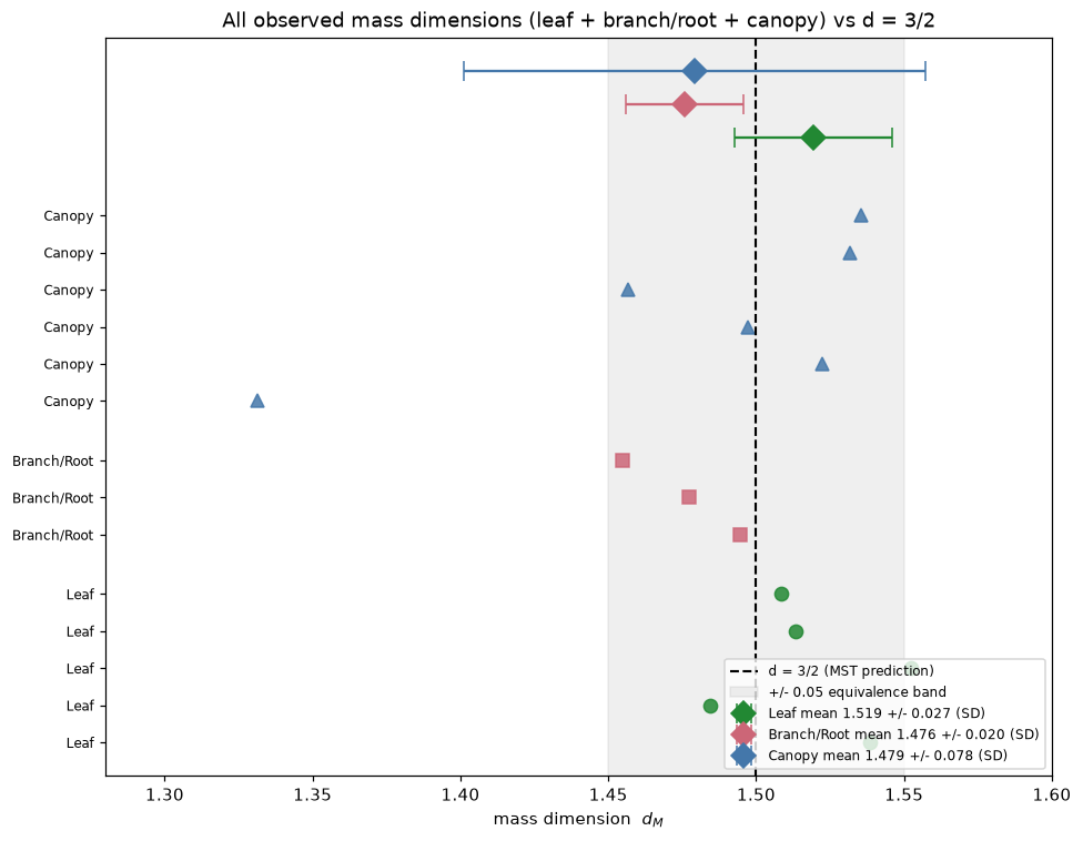
All 14 observed dimensions are shown against the \(d = 3/2\) reference line, with the \(\pm0.05\) equivalence band shaded and each group's mean \(\pm\) SD.

fig, ax = plt.subplots(figsize=(9, 7))
groups = [("Leaf", leaf_vals, "#228833", "o"),
          ("Branch/Root", branch_vals, "#cc6677", "s"),
          ("Canopy", canopy_vals, "#4477aa", "^")]
y = 0; yticks = []; ylabels = []
for label, arr, color, marker in groups:
    for v in arr:
        ax.plot(v, y, marker, color=color, ms=8, alpha=0.85)
        yticks.append(y); ylabels.append(label); y += 1
    y += 0.6

ax.axvline(1.5, ls="--", color="black", lw=1.4, label="d = 3/2 (MST prediction)")
ax.axvspan(1.45, 1.55, color="gray", alpha=0.12, label="+/- 0.05 equivalence band")

# group means with SD bars, placed at the top
ytop = y + 0.5
for label, arr, color, marker in groups:
    m = arr.mean(); sd = arr.std(ddof=1)
    ax.errorbar(m, ytop, xerr=sd, fmt="D", color=color, capsize=6, ms=10,
                label=f"{label} mean {m:.3f} +/- {sd:.3f} (SD)")
    ytop += 0.9

ax.set_yticks(yticks); ax.set_yticklabels(ylabels, fontsize=8)
ax.set_xlabel("mass dimension  $d_M$"); ax.set_xlim(1.28, 1.60)
ax.set_title("All observed mass dimensions (leaf + branch/root + canopy) vs d = 3/2")
ax.legend(fontsize=8, loc="lower right"); fig.tight_layout(); plt.show()

Figure 1: output of code cell 10

Summary¶

What was reproduced / verified (computed):

Table 4 (6 forest CHM sites) transcribed verbatim; canopy mean \(= 1.4791\), SD \(= 0.0781\), matching the manuscript's \(1.479 \pm 0.080\).
Group means reproduce the manuscript: leaf \(1.5194\), branch/root \(1.4757\), canopy \(1.4791\).
One-sample \(t\)-tests against \(1.5\): no group's mean is significantly different from \(3/2\) at \(\alpha = 0.05\) (leaf \(p \approx 0.18\), branch \(p \approx 0.17\), canopy \(p \approx 0.54\)); the pooled mean \(1.4928\) is statistically indistinguishable from \(1.5\) (\(p \approx 0.63\)).
TOST equivalence (\(\alpha = 0.05\)): at margin \(\pm 0.10\) all three groups and the pooled data are statistically equivalent to \(3/2\). At the stricter \(\pm 0.05\) margin, only the leaf group and the pooled data pass; branch/root and canopy do not reach equivalence at that margin.

Honest interpretation:

Canopy and leaf dimensions straddle \(1.5\) (leaf mean slightly above, canopy essentially on it). Branch/root sits a little below \(1.5\) (mean \(1.476\)), consistent with the manuscript's own framing.
The pooled data support the MST prediction at the \(\pm 0.10\) margin, but the stricter \(\pm 0.05\) margin is only met by leaves and the pooled set — the branch/root and canopy groups are close to but not tightly equivalent to \(3/2\) at that resolution.

What is asserted vs computed:

The Table 4 \(d_M\), \(\mu r^2\), pixel counts, and site identities are asserted from the manuscript (the authors' FracLac output on their LiDAR CHMs; raw rasters not in the repository).
Every mean, SD, SE, \(t\)-statistic, \(p\)-value, and TOST result is computed here with scipy.stats.

Caveats:

Group sizes are small (\(n = 5, 3, 6\); pooled \(14\)), so both the \(t\)-tests (low power) and the TOST (wide equivalence bounds) are limited in resolution. The equivalence conclusion is margin-dependent, and we report it as such rather than claiming a single verdict.