Foundations of Fractal Geometry
Jupyter notebook
This page was rendered from the stored outputs of fractals.ipynb as of 2026-10-24; it is not executed at build time.
View on GitHub · Open in nbviewer · Open in Colab · Raw .ipynb
Kernel: Python 3 · Environment: environments/fractal-foundations-gpu.yml (runs on CPU: numpy, matplotlib) · Companion page: foundations/
This notebook provides an overview of the Foundations section, with quick demonstrations and links to detailed notebooks.
Notebook Series
The Foundations section is organized into four chapters corresponding to the documentation:
| Notebook | Topics | Key Concepts |
|---|---|---|
| 1_history.ipynb | History of Fractal Mathematics | Cantor, Koch, Sierpinski, Julia, Mandelbrot, Weierstrass |
| 2_mathematics.ipynb | Mathematical Foundations | Box-counting, DBC, power laws, Hurst exponent, lacunarity |
| 3_dimensionality.ipynb | Fractal Dimensionality (1D-4D) | Pink noise, fBm, Mandelbrot/Julia, Menger, DLA |
Quick Start: Essential Fractals
Below are minimal examples of key fractal types. See the specialized notebooks for detailed explanations and analyses.
import numpy as np
import matplotlib.pyplot as plt
from matplotlib.patches import Polygon
from matplotlib.collections import PatchCollection

plt.rcParams['figure.figsize'] = [12, 8]
plt.rcParams['figure.dpi'] = 100
1D Fractals: Cantor Set
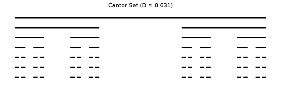
The Cantor set (1883) iteratively removes the middle third of each interval.
Dimension: \(D = \frac{\log 2}{\log 3} \approx 0.631\)
See 1_history.ipynb for detailed exploration.
def cantor_set(ax, x, y, length, depth, max_depth):
    """Draw Cantor set recursively."""
    ax.plot([x, x + length], [y, y], color='black', lw=3)
    if depth < max_depth:
        new_length = length / 3
        cantor_set(ax, x, y - 0.12, new_length, depth + 1, max_depth)
        cantor_set(ax, x + 2 * new_length, y - 0.12, new_length, depth + 1, max_depth)

fig, ax = plt.subplots(figsize=(12, 4))
cantor_set(ax, 0, 1, 1, 0, 6)
ax.set_xlim(-0.05, 1.05)
ax.set_ylim(0, 1.1)
ax.set_title(f'Cantor Set (D ≈ {np.log(2)/np.log(3):.3f})', fontsize=14)
ax.axis('off')
plt.show()
2D Fractals: Sierpinski Triangle
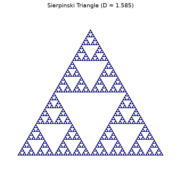
The Sierpinski triangle (1915) removes the central triangle at each iteration.
Dimension: \(D = \frac{\log 3}{\log 2} \approx 1.585\)
See 1_history.ipynb for construction details and 3_dimensionality.ipynb for chaos game implementation.
def sierpinski_triangle(ax, vertices, depth, patches):
    """Generate Sierpinski triangle."""
    if depth == 0:
        patches.append(Polygon(vertices, closed=True))
    else:
        midpoints = [(vertices[i] + vertices[(i + 1) % 3]) / 2 for i in range(3)]
        sierpinski_triangle(ax, np.array([vertices[0], midpoints[0], midpoints[2]]), depth-1, patches)
        sierpinski_triangle(ax, np.array([vertices[1], midpoints[1], midpoints[0]]), depth-1, patches)
        sierpinski_triangle(ax, np.array([vertices[2], midpoints[2], midpoints[1]]), depth-1, patches)

fig, ax = plt.subplots(figsize=(8, 7))
vertices = np.array([[0, 0], [1, 0], [0.5, np.sqrt(3)/2]])
patches = []
sierpinski_triangle(ax, vertices, 6, patches)
collection = PatchCollection(patches, facecolor='darkblue', edgecolor='black', linewidth=0.2)
ax.add_collection(collection)
ax.set_xlim(-0.1, 1.1)
ax.set_ylim(-0.1, 1)
ax.set_aspect('equal')
ax.set_title(f'Sierpinski Triangle (D ≈ {np.log(3)/np.log(2):.3f})', fontsize=14)
ax.axis('off')
plt.show()
3D Fractals: Menger Sponge
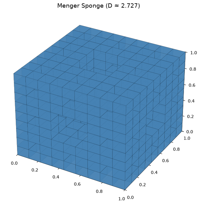
The Menger sponge (1926) is the 3D analog of the Sierpinski carpet.
Dimension: \(D = \frac{\log 20}{\log 3} \approx 2.727\)
See 3_dimensionality.ipynb for 3D visualization.
from mpl_toolkits.mplot3d.art3d import Poly3DCollection

def menger_cubes(x, y, z, size, depth):
    """Generate Menger sponge cube positions."""
    if depth == 0:
        return [(x, y, z, size)]
    new_size = size / 3
    cubes = []
    for dx in range(3):
        for dy in range(3):
            for dz in range(3):
                if (dx == 1) + (dy == 1) + (dz == 1) >= 2:
                    continue
                cubes.extend(menger_cubes(x + dx*new_size, y + dy*new_size, z + dz*new_size, new_size, depth-1))
    return cubes

def draw_cube(ax, x, y, z, size):
    v = np.array([[x, y, z], [x+size, y, z], [x+size, y+size, z], [x, y+size, z],
                  [x, y, z+size], [x+size, y, z+size], [x+size, y+size, z+size], [x, y+size, z+size]])
    faces = [[v[0],v[1],v[2],v[3]], [v[4],v[5],v[6],v[7]], [v[0],v[1],v[5],v[4]],
             [v[2],v[3],v[7],v[6]], [v[1],v[2],v[6],v[5]], [v[0],v[3],v[7],v[4]]]
    ax.add_collection3d(Poly3DCollection(faces, facecolors='steelblue', linewidths=0.1, edgecolors='black', alpha=0.8))

fig = plt.figure(figsize=(10, 8))
ax = fig.add_subplot(111, projection='3d')
for x, y, z, size in menger_cubes(0, 0, 0, 1, 2):
    draw_cube(ax, x, y, z, size)
ax.set_xlim(0, 1); ax.set_ylim(0, 1); ax.set_zlim(0, 1)
ax.set_title(f'Menger Sponge (D ≈ {np.log(20)/np.log(3):.3f})', fontsize=14)
plt.show()
Self-Affine Fractals: Fractional Brownian Motion
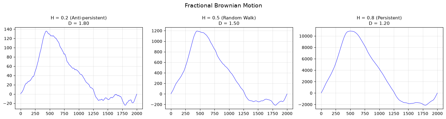
Fractional Brownian motion (fBm) is parameterized by the Hurst exponent \(H\): - \(H < 0.5\): Anti-persistent (mean-reverting) - \(H = 0.5\): Standard Brownian motion - \(H > 0.5\): Persistent (trending)
Dimension: \(D = 2 - H\)
See 2_mathematics.ipynb for Hurst exponent estimation and 3_dimensionality.ipynb for detailed analysis.
def generate_fbm(n, H, seed=42):
    """Generate fractional Brownian motion."""
    np.random.seed(seed)
    freqs = np.fft.rfftfreq(n)
    freqs[0] = 1e-10
    spectrum = 1.0 / np.abs(freqs) ** ((2*H + 1) / 2)
    spectrum[0] = 0
    phases = np.exp(2j * np.pi * np.random.rand(len(freqs)))
    return np.cumsum(np.fft.irfft(spectrum * phases, n))

fig, axes = plt.subplots(1, 3, figsize=(15, 4))
for i, H in enumerate([0.2, 0.5, 0.8]):
    fbm = generate_fbm(2000, H)
    axes[i].plot(fbm, 'b-', lw=0.7)
    behavior = 'Anti-persistent' if H < 0.5 else ('Persistent' if H > 0.5 else 'Random Walk')
    axes[i].set_title(f'H = {H} ({behavior})\nD = {2-H:.2f}', fontsize=11)
    axes[i].grid(True, alpha=0.3)
fig.suptitle('Fractional Brownian Motion', fontsize=14)
plt.tight_layout()
plt.show()
Fractal Dimension Reference
| Fractal | N copies | Scale r | Dimension D |
|---|---|---|---|
| Cantor Set | 2 | ⅓ | 0.631 |
| Koch Curve | 4 | ⅓ | 1.262 |
| Sierpinski Triangle | 3 | ½ | 1.585 |
| Sierpinski Carpet | 8 | ⅓ | 1.893 |
| Menger Sponge | 20 | ⅓ | 2.727 |
Formula: \(D = \frac{\log N}{\log(1/r)}\)
print("Self-Similar Fractal Dimensions")
print("=" * 50)
fractals = [
    ("Cantor Set", 2, 3),
    ("Koch Curve", 4, 3),
    ("Sierpinski Triangle", 3, 2),
    ("Sierpinski Carpet", 8, 3),
    ("Menger Sponge", 20, 3),
]
for name, N, inv_r in fractals:
    D = np.log(N) / np.log(inv_r)
    print(f"{name:<22} D = log({N})/log({inv_r}) = {D:.4f}")
Self-Similar Fractal Dimensions
==================================================
Cantor Set             D = log(2)/log(3) = 0.6309
Koch Curve             D = log(4)/log(3) = 1.2619
Sierpinski Triangle    D = log(3)/log(2) = 1.5850
Sierpinski Carpet      D = log(8)/log(3) = 1.8928
Menger Sponge          D = log(20)/log(3) = 2.7268
Next Steps
For deeper exploration:
-
1_history.ipynb - Historical development: Cantor, Koch, Sierpinski, Julia, Mandelbrot, Weierstrass function
-
2_mathematics.ipynb - Measurement methods: box-counting, differential box-counting, power law analysis, Hurst exponent, lacunarity
-
3_dimensionality.ipynb - Examples across dimensions: 1D (pink noise, fBm), 2D (Mandelbrot/Julia, fBs), 3D (Menger, DLA), 4D (growth dynamics)
Related sections:
- biological-geometry/ - Branching architectures, vascular networks, L-systems
- metabolic-scaling/ - West-Brown-Enquist theory, allometric scaling